Hi people, it’s me again.
Some notes on the “Programming Assignment 1” for “Week 1” on “Initialization”
Behind the scenes
In the provided file init_utils.py we find a “non-vectorized” external loop (comments elided):
def predict(X, y, parameters):

    m = X.shape[1]
    p = np.zeros((1,m), dtype = np.int)

    a3, caches = forward_propagation(X, parameters)

    for i in range(0, a3.shape[1]):
        if a3[0,i] > 0.5:
            p[0,i] = 1
        else:
            p[0,i] = 0

    print("Accuracy: "  + str(np.mean((p[0,:] == y[0,:]))))

    return p
There is occasion to replace the external loop with a call to np.rint()
p = np.rint(a3)
Loading the datatset
It is a bit obscure what the dataset is.
Why not be explicit by adding this note:
The dataset is a randomly generated set of 2D points arranged in two concentric circles, with class
0, the “red dots” enclosing the smaller circle of class1, the blue dots.They have been created with the
make_circles()function. See the SciKit-Learn manual under Generated datasets
And then be somewhat more talkative in the code:
train_X, train_Y, test_X, test_Y = load_dataset()

# X numpy arrays contains 2 coordinates (x,y)
# Y numpy arrays contains integer labels for classes: 0 for "red dots", 1 for "blue dots"

num_train_examples = train_X.shape[1]
num_test_examples = test_X.shape[1]

assert train_X.shape == (2, num_train_examples), f"Shape of train_X is {train_X.shape}"
assert test_X.shape == (2, num_test_examples), f"Shape of test_X is {test_X.shape}"

assert train_Y.shape == (1, num_train_examples), f"Shape of train_Y is {train_Y.shape}"
assert test_Y.shape == (1, num_test_examples), f"Shape of test_Y is {test_Y.shape}"

plt.axis('equal') # aspect ratio 1:1
plt.show()
3 Neural Network Model
There is text error
Instructions: Instructions:
Easy fix.
The function compute_loss() should be called compute_cost()
The function definition for compute_loss() in init_utils.py clearly computes the cost/J. And is used as such in model(), originally:
        # Loss
        cost = compute_loss(a3, Y)
The plot is somehow auto-adapting
This may be nothing but I didn’t understand the plot when playing around with small deltas in the gradient. Apparently pyplot plots the differences from ln(2) if all the values (the costs) are near ln(2). This is also why the plot displays a cost value in its upper left. Maybe a note here could help.
The original plot code, moved out into a function, is:
def plot1(costs, learning_rate):
    plt.plot(costs)
    plt.ylabel('cost')
    plt.xlabel('iterations (per hundreds)')
    plt.title("Learning rate =" + str(learning_rate))
    plt.yscale('linear')
    plt.show()
The modified plot code, moved out into a function, is:
def plot2(costs, learning_rate):
    plt.plot(costs, marker='o', linestyle='-')
    plt.ylim(min(costs) - 1e-10, max(costs) + 1e-10)
    plt.ticklabel_format(style='plain', axis='y')  # Avoid scientific notation
    plt.ylabel("cost")
    plt.xlabel('iterations (per hundreds)')
    plt.title("Learning rate =" + str(learning_rate))
    ax = plt.gca()
    ax.yaxis.set_major_formatter(ScalarFormatter(useOffset=False))
    plt.grid(True)
    plt.show()
Calling the above after training (with zero initialization but with “rattling” where the update is disturbed by a random numbers) brings for example:

IN case of pure zero initialization:

What’s this “rattling” thing you ask? Simple, in init_utils.py, modify the update_parameters() like so:
def update_parameters(parameters, grads, learning_rate, rattle=0.0):

    L = len(parameters) // 2 # number of layers in the neural networks

    # Update rule for each parameter
    for k in range(1,L+1):
        parameters[f"b{k}"] += -learning_rate * grads[f"db{k}"]
        parameters[f"W{k}"] += -learning_rate * grads[f"dW{k}"]
        if rattle > 0.0:
            wshape = parameters[f"W{k}"].shape
            parameters[f"W{k}"] += rattle * np.random.randn(*wshape)

    return parameters
and then update parameters in the main loop like this for example:
parameters = update_parameters(parameters,
  grads,
  learning_rate,
  rattle/(np.sqrt(i+1.0))) # decay the rattle
rattle is passed to model() as named parameter for maximal ease of use:
def model(X, Y, learning_rate = 0.01,
 num_iterations = 15000, print_cost = True,
 initialization = "he", rattle = 0.0):
A zero initialization with a “rattle” at high 0.1 with the decay 1/sqrt(i) given above and a lot more training iterations kinda works, but in the end, it’s no different from random initialization (or is it)?
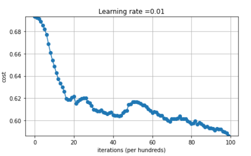
In the above the x axis is wrong by a factor 10 for some reason. ![]()
4 Zero Initialization
Give link
As usual one may want to give a link directly to the numpy manual:
Change:
# layer_dims -- python array (list) containing the size of each layer.
to:
# layer_dims -- python array (list) containing the size of each layer, including the input layer
Erroneous comment, unfortunate loop
After that, the comment for the loop is wrong.
This applies also to the subsequent “random initialization”.
But it is correct for “He initialization”.
The wrong comment and unfortunately chosen loop limits:
L = len(layers_dims)            # number of layers in the network

    for l in range(1, L):
L is the number of layers + 1, not the number of layers.
The code for He initialization does it exactly right:
L = len(layers_dims) - 1 # integer representing the number of layers

    for l in range(1, L + 1):
so I recommend just doing it like for He in all cases.
Explainer improvements
The explanation for why we are stuck has this text:
As you can see with the prediction being 0.5 whether the actual (
y) value is 1 or 0 you get the same loss value for both, so none of the weights get adjusted and you are stuck with the same old value of the weights.
But the fact that the loss is equal for all labels is not the problem. The problem is that the gradient of the error is 0 in all components (except db3, so we are wiggling a bit there) - in all w's from all layers and all b's from all layers, and it stays that way.
This can be easily seen by taking my preferred diagram (for a 2-layer network though) and just tracing backward - everything is 0 everywhere and it stays that way. This is also explained “Paul Mielke’s post”

In fact, here is simple addition to add to the model function to show this, directly after calling back_propagation() (properly moved this to a separate function to not smother the loop):
def printing(print_cost, i, grads):
    if print_cost and i % 1000000 == 0:
        for name in ['dz3', 'dW3', 'db3',
                     'da2', 'dz2', 'dW2', 'db2',
                     'da1', 'dz1', 'dW1', 'db1']:
            arr = grads[name]
            if np.unique(arr).size == 1:
                print(f"{name}({i}) of shape {arr.shape} contains {arr[0, 0]} everyhwere")
            else:
                absarr = np.abs(arr)
                if np.unique(absarr).size == 1:
                    print(f"{name}({i}) of shape {arr.shape} contains +/-{np.abs(arr[0, 0])} everyhwere")
                else:
                    testval = absarr[0, 0]
                    if np.all(np.isclose(absarr, testval, atol=0.000000001)):
                        print(f"{name}({i}) of shape {arr.shape} contains approx +/-{testval} everyhwere")
                    else:
                        print(f"{name}({i}) of shape {arr.shape} is {arr}")
And then in the loop of model(), call the above:
        # Backward propagation.
        grads = backward_propagation(X, Y, cache)

        printing(print_cost, i, grads)
When running the training, one sees:
dz3(7000) of shape (1, 300) contains +/-0.0016666666666666668 everyhwere
dW3(7000) of shape (1, 5) contains 0.0 everyhwere
db3(7000) of shape (1, 1) contains -2.6020852139652106e-18 everyhwere
da2(7000) of shape (5, 300) contains 0.0 everyhwere
dz2(7000) of shape (5, 300) contains 0.0 everyhwere
dW2(7000) of shape (5, 10) contains 0.0 everyhwere
db2(7000) of shape (5, 1) contains 0.0 everyhwere
da1(7000) of shape (10, 300) contains 0.0 everyhwere
dz1(7000) of shape (10, 300) contains 0.0 everyhwere
dW1(7000) of shape (10, 2) contains 0.0 everyhwere
db1(7000) of shape (10, 1) contains 0.0 everyhwere
Cost after iteration 7000: 0.6931471805599453
5 Random Initialization
Give link
As usual one may want to give a link directly to the numpy manual:
Recommending changing the comment
As above
Erroneous comment, unfortunate loop
As above
Typo in the comment after np.random.seed(3)
Easy fix
Probably erroneous explainer
We read:
If you see “inf” as the cost after the iteration 0, this is because of numerical roundoff.
More like
If you see
infas the cost after the iteration 0, this is because of numerical overflow (because we computelog(0))
Unclear explainer
We read:
You’ll remember that the slope near 0 or near 1 is extremely small, so the weights near those extremes will converge much more slowly to the solution, and having most of them near the center will speed the convergence.
The weights are certainly not near the extremes. That should probably be:
You’ll remember that the slope near 0 or near 1 is extremely small, so if the
avalues are near those extremes, gradients will be near 0 and weights will converge much more slowly to a solution. Havingzvalues around 0 and thusavalues near 1/2 in the last layer will speed the convergence.
6 - He Initialization
Why not give links to the papers? They are quite fascinating.
2010-01: “Understanding the difficulty of training deep feedforward neural networks”, Xavier Glorot, Yoshua Bengio.
Proceedings of Machine Learning research
2015-06: “Delving Deep into Rectifiers: Surpassing Human-Level Performance on ImageNet Classification”, Kaiming He, Xiangyu Zhang, Shaoqing Ren, Jian Sun
Arxiv
And now a discussion about whether the correct naming is chosen.
In Glorot/Bengio, the authors say the “commonly used heuristic” is choosing a value from the uniform distribution over the interval (equation 1):
[- \frac{1}{\sqrt{n_{j}}}, +\frac{1}{\sqrt{n_{j}}}]
where n_{j} is the width of the previous layer. The weights may be scaled.
This gives bad convergence. The authors then proceed to develop and propose choosing from the uniform distribution over the following interval (equation 16):
[- \frac{\sqrt{6}}{\sqrt{n_{j} + n_{j+1}}}, +\frac{\sqrt{6}}{\sqrt{n_{j} + n_{j+1}}}]
The weights may be scaled.
However, what we call “Xavier Initialization” (also in the presentation under “Weight Initialization for Deep Networks / Single Neuron Example”), is apparently (when using tanh):
- Choosing from the normal distribution and then
- scaling by \sqrt{\frac{1}{n_{j}}}, sometimes \sqrt{\frac{2}{n_{j} + n_{j+1}}}
i.e. the result is choosing from a normal distribution with mean zero and standard deviation \sqrt{\frac{1}{n_{j}}}, or \sqrt{\frac{2}{n_{j} + n_{j+1}}}
Not the same at all. Why do we call the latter “Xavier initialization” then?
Also, in He, Zang et al. (working with ReLU) we find, after equation 14, that they propose sampling from the normal distribution with standard deviation \sqrt{\frac{2}{n_{j}}} (if I understand well), so “He initialization” would be choosing from a wider distribution.
This is also the correct formula given in the exercise.